COVID-19 Time-Varying Reproduction Numbers on Global
Background and Motivation
Currently, COVID-19 has become a global scale threat to our health. Meanwhile, the situation in some regions such as China and Singapore has more or less become stable. To help everyone to be more aware of the global situation, and even hopefully contribute our possibly 3 cents to intervention of this epidemics, we here calculated the time-varying reproduction number from time series of case numbers in each region on which we can get data and share it on this website. We will update daily when possible.
The basic reproduction number [math]\displaystyle{ R_{0} }[/math], which means roughly the number of new individuals will be infected on average by a single infector when there is no intervention at all, and the corresponding time-varying reproduction number [math]\displaystyle{ R\left(t\right) }[/math] at time [math]\displaystyle{ t }[/math] with possibly some interventions, are two important indicators of how severe is the epidemics and how effective are the interventions.
Here, we will provide first a time series of [math]\displaystyle{ R\left(t\right) }[/math] for each region on which we get data, and we will also show some predictive results based on very simple and rough extensions, which will be explained in the following.
Methods
While working on analysis of COVID-19 data, we note that the effective time-varing reproduction number of imported cases ([math]\displaystyle{ R_{0}^{1}\left(t\right) }[/math]) can be very different from the one of local cases ([math]\displaystyle{ R_{1+}^{2+}\left(t\right) }[/math]) due to the different intervention policy for imported cases and local cases. Thus, we
- classfifed all cases into the imported cases (the zeroth generation)[math]\displaystyle{ I^{0}\left(t\right) }[/math], locals infected by the imported cases (first generation) [math]\displaystyle{ I^{1}\left(t\right) }[/math] and locals infected by locals (second generation and beyond) [math]\displaystyle{ I^{2+}\left(t\right) }[/math],
- derived formulea calculating [math]\displaystyle{ R_{0}^{1}\left(t\right), R_{1+}^{2+}\left(t\right) }[/math] from time series of [math]\displaystyle{ I^{0}\left(t\right), I^{1}\left(t\right), I^{2+}\left(t\right) }[/math],
- Modified the R software EpiEstim according to the newly derived formulea.
Also, the test version of the modified EpiEstim has been provided at Github, and the manuscript on this new calculation will soon be posted on an arXiv website.
With the calculated [math]\displaystyle{ R\left(t\right) }[/math], we constructed two simple and rough scenarios to make some prediction,
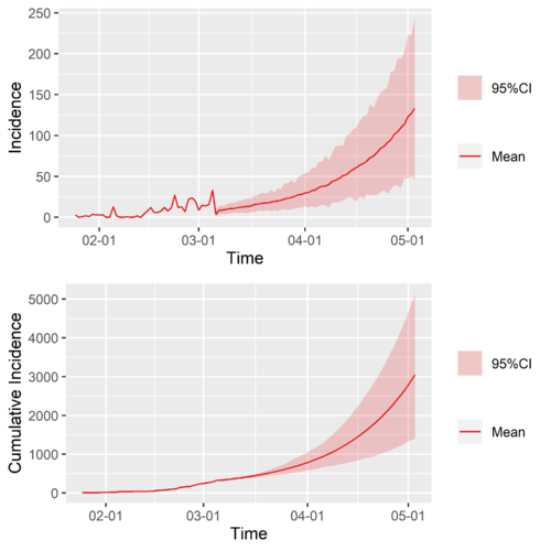
- Null Scenario: extend the [math]\displaystyle{ R\left(t\right) }[/math] of a region of interest by taking [math]\displaystyle{ R\left(t\gt t_{end}\right)=R\left(t\gt t_{end}\right) }[/math], where [math]\displaystyle{ t_{end} }[/math] is the latest time of the known [math]\displaystyle{ R\left(t\right) }[/math], that is to say just take the latest value to be the future value of the time-varying reproduction number of a region of interest,
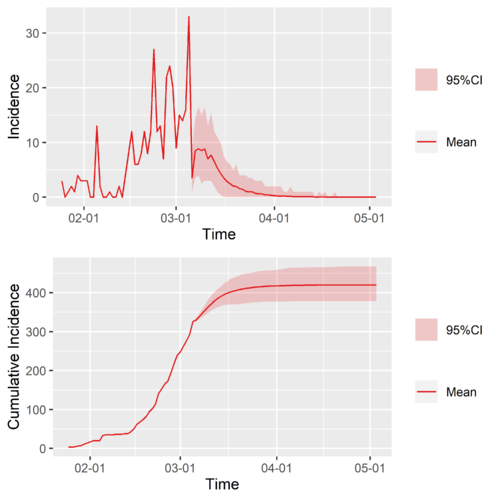
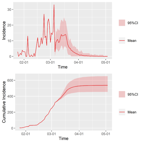
- Typical-Region Scenario: Extend the [math]\displaystyle{ R\left(t\right) }[/math] of a region of interest by connecting to it the [math]\displaystyle{ R_{typical}\left(t\right) }[/math] of a chosen typical region, which we use China (cn) and Singapore (sg).
[math]\displaystyle{ R\left(t\right) }[/math] of the two typical regions are decreasing functions since there is no data at the very beginning and when there are data, usually there are interventions already.
When we connect for example [math]\displaystyle{ R_{cn}\left(t\right) }[/math] to [math]\displaystyle{ R\left(t\right) }[/math] of a region of interest, we might encouter three cases. Firstly, if the latest value [math]\displaystyle{ R\left(t_{end}\right) }[/math] is smaller than some values but at all values of [math]\displaystyle{ R_{cn}\left(t\right) }[/math], we find the place [math]\displaystyle{ t_{0} }[/math] such that [math]\displaystyle{ R_{cn}\left(t_{0}\right)=R\left(t_{end}\right) }[/math] and then let [math]\displaystyle{ R\left(t_{end}+t\right)=R_{cn}\left(t_{0}+t\right) }[/math]. Secondly, if the latest value [math]\displaystyle{ R\left(t_{end}\right) }[/math] is larger than all values of [math]\displaystyle{ R_{cn}\left(t\right) }[/math], we left extrapolate [math]\displaystyle{ R_{cn}\left(t\right) }[/math] (for example using the splinefun R function) so that we will find a large enough value such that [math]\displaystyle{ R_{cn}\left(t_{0}\right)=R\left(t_{end}\right) }[/math] (here [math]\displaystyle{ t_{0}\lt 0 }[/math]) and then again we let [math]\displaystyle{ R\left(t_{end}+t\right)=R_{cn}\left(t_{0}+t\right) }[/math]. Lastly, in principle, there is a case where [math]\displaystyle{ R\left(t_{end}\right) }[/math] is smaller than all [math]\displaystyle{ R_{cn}\left(t\right) }[/math], but we have not see such a cases in real data.
The Null Scenario is like to ask that if nothing changes what will happen, while the Typical-Region Scenario is to ask when will happen if the region of interest learn from the typical regions and those learned interventions are exactly as effective as they were in the original region.
There are some limitations of the method. First, the scenarios are too simple to be realistic. Second, in many other regions, due to data limitations, we have not distinguished the zeroth, first, second and beyond generations of cases. The method is currently applied to a single-region model, where all the other regions are treated as exogenous variables. In principle, the method is readily applicable to a multi-region situation, where flows among the regions can be estimated via traffic data.
Appendex to the methods section: some core formulea
If you are interested in knowing more about our analysis before we publish the paper, here are some core formulea:
- Locals infected by imported cases from some specific regions [math]\displaystyle{ I^{1}\left(t\right)=\sum_{\tau=0}^{\infty}I^{0}\left(t-\tau\right)R_{0}^{1}\left(t\right)\omega\left(\tau\right) }[/math], where the zeroth generation refers to the imported cases and locals infected by them are called the first generation
- Locals infected by local infectors, which themselves can be from the first generation or beyond [math]\displaystyle{ I^{2+}\left(t\right)=\sum_{\tau=0}^{\infty}\left(I^{1}\left(t-\tau\right)+I^{2+}\left(t-\tau\right)\right)R_{1+}^{2+}\left(t\right)w\left(\tau\right) }[/math], which we call the second generation and beyond
Correspondingly the time-varying reproducton numbers are respectively,
- [math]\displaystyle{ R_{0}^{1}\left(t\right)=\frac{I^{1}\left(t\right)}{\sum_{\tau=0}^{\infty}I^{0}\left(t-\tau\right)\omega\left(\tau\right)} }[/math]
- [math]\displaystyle{ R_{1+}^{2+}\left(t\right)=\frac{I^{2+}\left(t\right)}{\sum_{\tau=0}^{\infty}\left[I^{1}\left(t-\tau\right)+I^{2+}\left(t-\tau\right)\right]w\left(\tau\right)} }[/math]
Time-varying reproduction number of typical regions
中国中国除去湖北之外的地区的再生数,以及,新加坡的再生数时间序列是将来做外推计算的基础。我们先把结果放在这里。
典型地区一:中国除去湖北之外的再生数
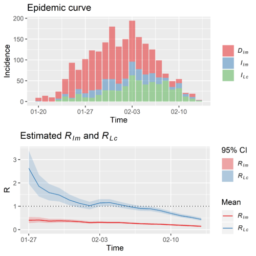
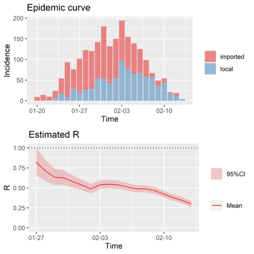
我们区分了中国湖北之外的数据中的输入、输入感染、本地感染三种病人,用发展了的方法做了有效再生数的计算。顺便,注意区分三种病人和不区分得到的再生数时间学列的结果相差非常大。
中国湖北之外的再生数,区分输入、输入感染、本地感染三种病人的计算
中国湖北之外的再生数,区分输入、本地两种病人的计算
注意,我们的新冠肺炎联合研究小组“公共安全和复杂系统”的学生处理了识别输入、输入感染、本地感染三种病人的数据。如果你有其他研究需要这个数据,请和我们联系。
典型地区二:新加坡的再生数
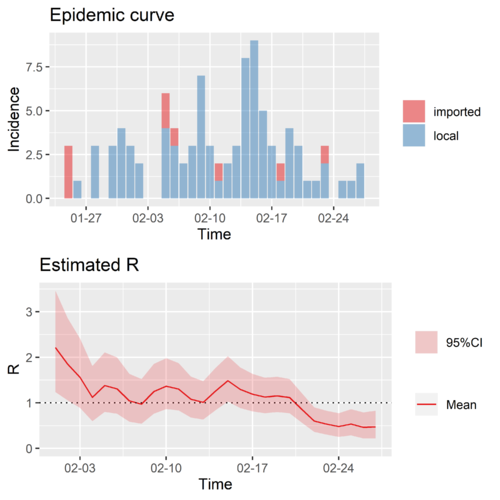
这是新加坡的再生数时间序列。由于数据限制,没有输入和本地病人。
各个国家的有效再生数时间序列以及简单外推的预测结果
下面,我们展示各个国家的再生数时间序列,以及我们简单外推的预测结果。
日本的再生数时间序列和外推预测
日本再生数时间序列
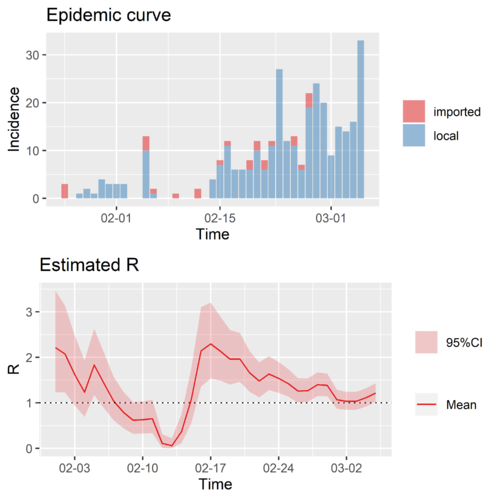
日本的再生数,未区分输入和本地病人
日本简单外推预测
日本再生数末位值外推结果
日本用中国和新加坡再生数时间序列接上得到的预测
日本用中国再生数时间序列接上的结果
日本用新加坡再生数时间序列接上的结果
